Fourier Series Approximations and Low Pass Filtering: Facilitating Learning of Digital Signal Processing for Biomechanics Students Steven J Elmer and James C Martin Sportscience 13, 1-8, 2009 (sportsci.org/2009/sjejcm.htm) |
|
Update 5
Sept 15: The
first spreadsheet was in xls format for Excel 2003 and earlier. We recently
became aware that the scroll bars were not working in more current versions of
Excel. We have added an updated spreadsheet in xlsx format which should
function properly in Excel 07-13. Update 3 April 10: The Butterworth, Velocity and Acceleration,
and Comparison spreadsheets now include sliding scroll bars to change the
cutoff frequency rapidly and sequentially.
This change should enhance the learning experience. Update 13
June 09: Correction
of expressions for the 2nd and Nth order Fourier approximations in the
article. Spreadsheet needed no
correction. Filtering raw biomechanical data (e.g., position, ground reaction force) to remove noise is a key first step that must be performed prior to further analysis such as determining velocity and acceleration or performing inverse dynamic calculations of joint torque. Most techniques for filtering raw biomechanical data are designed to remove noise above (low pass filtering) or below (high pass filtering) a specified cutoff frequency. Although low frequency noise and high pass filtering are used in some biomechanical applications (e.g., EMG) this paper and the related spreadsheet will deal only with low pass filtering and will use the Butterworth low-pass filter (Winter, 2005). Regardless of the type of filter used, the student must grasp the concept that data contain components that occur at various frequencies. Several authors of biomechanics textbooks (e.g., Enoka, 2008; Griffiths, 2006; Robertson et al., 2004; Winter, 2005) introduce the notion of frequency content in data within the context of a Fourier series approximation. This technique can be used to approximate data representing any movement cycle that occurs over a known time interval (T) or at a known frequency (f = 1/T) by summing a series of trigonometric functions (sine or cosine). For example, T might represent the time for one complete gait or pedal cycle and f would be the stride or pedaling frequency. Fourier series approximations are described in many textbooks and we recommend the reader consult a favorite math or biomechanics textbook for a full treatment of the topic. In this paper, we will provide a brief description and demonstrate Fourier series approximations using sample pedal reaction force (PRF) data in an Excel spreadsheet. The data represent a pedaling rate of 120 rpm, or a movement frequency of 2 Hz, and were recorded at a sampling rate of 240 Hz. The Excel spreadsheet includes columns for time, raw PRF data, approximated PRF data, and a squared error term (SE). Fourier series coefficients were determined iteratively by minimizing the sum of squared error (SSE) between the raw PRF data and the Fourier approximation. The Excel spreadsheet also includes a fourth-order zero-lag Butterworth filter with adjustable cutoff frequency. In one tab (“Comparison”), the filtered PRF data can be compared to several orders of Fourier series approximations. Finally, a set of kinematic data was used to illustrate the importance of filtering when data are to be differentiated to determine velocity and acceleration terms. We have used this Excel spreadsheet to teach graduate and honors undergraduate biomechanics courses and have found that it facilitates hands-on learning of a topic that can be quite abstract. We believe that this paper and related Excel spreadsheet will be useful as a teaching tool in higher education and will be helpful for anyone interested in analyzing biomechanical data who does not have a strong background in digital signal processing. The Excel spreadsheet may also be helpful to many other spreadsheet users because it demonstrates a general method for determining any type of regression coefficients (including non-linear) using the first-principles approach of minimizing sum of squared error. Please note that this spreadsheet and the instructions were derived using Excel from Office 2003 and newer versions of Excel may function differently. Also, help with the solver function is available from this link at the Microsoft website. Fourier
Series Approximation
Zero Order
The most basic approximation to a signal (e.g., position, force) is the mean of that signal over the entire time interval. In the Fourier series approximation the mean is referred to as the zero order approximation and given the coefficient a0. A zero order approximation to a signal would be written, for example, as X(t) = a0, where t represents time. The mean will give some information about the signal but it will provide no detail about the variation of the signal within the movement (at any specific point in time). Thus, the a0 coefficient is not generally used by itself but rather in combination with higher order coefficients. First
Order and Basic Ideas
Many movement patterns are generally sinusoidal in nature (e.g., limb kinematics during gait) and thus a sine function may provide a reasonable approximation to the movement: X(t) = sin(t). In this case, the time variable “t” refers to the instantaneous time at a point within the movement. That time value must be scaled to the overall time (T) or frequency (f = 1/T) of the movement (Figure 1). That is, instead of absolute time, the expression for the sine function must represent t/T to represent a relative time within the cycle. Further, the input to a sine function must be an angle, so the time variable must be expressed as a portion of a complete angular cycle (2p) and the variable becomes 2pt/T so that X(t) = sin(2pt/T). In this way, a complete cycle of a sinusoid is generated as “t” goes from 0 to T. The signal might not oscillate equally above and below zero but rather above and below the mean value (a0) and thus the approximation will be improved by adding the mean to the sine function: X(t) = a0 + sin(2pt/T). The sine function must also be modified to take into account the amplitude (a1) of the movement (how far above and below the mean the movement oscillates; Figure 1) so the approximation becomes: X(t) = a0 + a1sin(2pt/T). Finally, the movement may not follow a true sine function in that it may not be zero at the initial point of the cycle. To correct for such an offset, the angle within the sine function should be corrected by adding some offset value q1 (Figure 1). Thus, the equation for a 1st order Fourier series approximation is: X(t) = a0 + a1sin(2pt/T+q1). This is termed a 1st order approximation, because it only includes the frequency of the overall movement. The meanings and functions of variables T, a0, a1, and q1 are illustrated in Figure 1.
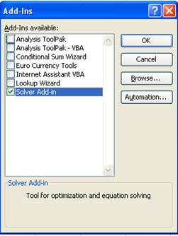
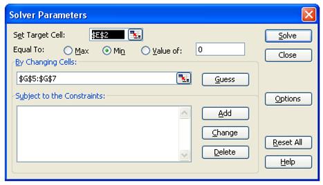
In the Excel spreadsheet, the tab labeled 1st Order illustrates this approximation. The coefficients (a0, a1, and q1) were determined iteratively using the Solver function in Excel. Note that the a0 coefficient determined by the Solver function is equal to the arithmetic mean of the raw data (shown in cell G9 of the 1st Order tab). The Solver function must be installed as an Add-in (Figure 2; select Tools menu; click Add-in, check Solver Add-in, click OK). The reader can examine the workings of this function by entering some other values in cells G5-G7 (e.g., 0’s) and then using Solver to achieve a minimum value of the sum of squared error term (SSE; cell E2; highlighted in red). Solver will do this by changing coefficient values in cells G5-G7 (highlighted in yellow) to minimize the sum of squared error term. From the tools menu select Solver and the Solver dialog box will appear (Figure 3). Once the correct cells and “Min” criterion are selected, click the solve button and the coefficients will be determined iteratively. Note that this first order approximation captures a great deal of the character of the PRF data with an r2 value of 0.94. Such a high agreement is characteristic for most kinetic and kinematic data associated with cycling, which is generally sinusoidal in nature. Other activities, such as gait, may be less well represented by the first order approximation.
Higher
Order Approximations
Fourier approximations are based on harmonics, or multiples of the central frequency of the movement. In this particular data set, the central frequency was 2 Hz. Thus each harmonic is 2 Hz and each multiple of that harmonic represents frequencies within the movement. That is, patterns that oscillate once within the movement occur at the central frequency, patterns that oscillate twice within the movement occur at twice the central frequency, and so on. In the spreadsheet tabs labeled 2nd Order, 3rd Order, 4th Order, and 10th Order, higher order Fourier series approximations have been formed for the same PRF data as used in the 1st order approximation. The higher order approximations include sinusoidal functions of additional multiples of the central or fundamental frequency. For example, the 2nd order approximation is calculated from the equation: X(t) = a0 + a1sin(2pt/T+q1) + a2sin(4pt/T+q2). The 4pt/T term in the second sine function represents the proportion of time within a cycle at twice the overall frequency of movement. Thus, the general form of the Fourier approximation for the Nth order is: X(t) = a0 + a1sin(2pt/T+q1) + a2sin(4pt/T+q2) + …+ aNsin(2Npt/T+qN). The additional frequencies allow the higher order approximations to follow additional nuances of the original signal. As series order is increased the approximations tend to converge upon the raw PRF data (Figure 4). Indeed, the 4th order approximation captures most of the nuances of the raw PRF data (r2 > 0.99). Because these PRF data have a movement frequency of 2 Hz, each additional order of approximation accounts for an additional 2 Hz in signal frequency content (2 Hz for the 1st order approximation, 4 Hz for the 2nd order, 6 Hz for the 3rd order, etc). As with the 1st order approximation, the reader can reset the coefficients to zero and use Solver to determine them again. Additional cells must be changed by the Solver tool for the higher order approximations (e.g., G5-G9 for 2nd Order, G5-G11 for 3rd Order, etc.) and in each tab the appropriate cells are highlighted with a yellow background. The appropriate cells should appear in the Solver dialog box (because they have been used previously in the building of the spreadsheet) but the reader should check that the cell references include all coefficients.
The spreadsheet can be used to examine the functions of the Fourier coefficients by performing the following exercise. In the 1st Order tab, reset the a0 coefficient to a vale of zero. When this change is made, the approximated data will oscillate about zero, rather than about the mean demonstrating that the a0 coefficient forces the approximation to vary about the mean. As mentioned above, the reader may note that the a0 coefficient is the same as the mean for the raw PRF data (cell G9). Once the effect has been observed, the reader may use the “undo” function (select edit; click on undo) to restore the coefficients or may use solver to reestablish them. Second, the reader may reset the a1 coefficient to zero and will note that the approximation becomes a straight line equal to the mean. This demonstrates that the a1 coefficient represents the amplitude of the excursion above and below the mean. Next, the reader may set the q1 coefficient to zero and will note that the approximated data is shifted horizontally relative to the raw data. This will demonstrate that the function of the q1 coefficient is to adjust the relative position of the sine function. These effects are also illustrated in Figure 1. Additionally, in the 2nd Order tab, setting the a1 coefficient to zero will reveal the effect of the a2 coefficient which causes the approximation to oscillate at twice the central frequency (twice with the movement cycle). This is only a brief exercise and the reader may wish to explore other coefficients and tabs. General
Method
We have used Solver to determine coefficients that minimize the sum of squared error term between the original data and the modeled approximation. This technique can be used to determine coefficients for any linear or non-linear approximation. To do this, one simply writes an equation for the model of choice which includes coefficients and independent variables (column “C” in our approximation spreadsheets). That equation should be “filled down” a column of an Excel spreadsheet so that an approximation is calculated for each data point. Further, a set of cells should be used as a location for the coefficients (column “G” in our spreadsheet). Any value can be selected for the initial coefficients (e.g., 0’s or 1’s). In the next column, one should form a squared error term as the difference in the raw value and the approximation squared (column “D” in our spreadsheet). All of these squared error terms are then summed to form the sum of squared error term (cell “E2” in our spreadsheet). Solver performs an iterative process to determine coefficient values that minimize this sum of squared error term. We have used this technique to determine coefficients for functions as basic as quadratic equations and as specialized as a Hill type force-velocity equation (rectangular hyperbola). The interested reader will likely find many applications for this technique. Butterworth
Filter
The fourth-order zero-lag Butterworth filter is often used in biomechanical analyses and is described in detail by Winter (2005). Briefly, this filter produces a weighted average of data from several time points and the weight on each time point (the a0, a1, a2, b1, b2 coefficients) determines the cutoff frequency (the frequency above which noise is removed). Note that these Butterworth coefficients are not related to the Fourier approximation coefficients of similar names. In our example filter, the weighted average includes the point of interest as well as the two preceding time points. This process of averaging time points prior to the time of interest causes the filtered data to “lag” behind the raw with respect to time. To correct for this lag, data are filtered once in forward time order, then again in reverse time order to produce filtered data that are properly aligned in time. In addition to correcting for lag, the second filtering in the reverse direction creates a sharper cutoff and this two-pass filter is referred to as a fourth-order zero-phase shift (or zero-lag) filter. We encourage the reader to consult a textbook (e.g., Winter 2005) for a thorough treatment of Butterworth filter. In the Excel spreadsheet tab labeled Butterworth, we have implemented just such a filter. We will not present the details of this filtering technique in this paper but rather provide it to illustrate the effects of filtering the PRF data at various cutoff frequencies and to allow the reader to explore the similarities and differences between Fourier series approximations and filtered data. The Butterworth coefficients (K1, K2, K3, a0, a1, a2, b1, b2) are calculated in the spreadsheet as described by Winter (2005, page 47). The a and b coefficients are the weights applied to the data. The K coefficients are used to calculate the a and b coefficients based on the desired cutoff frequency and the known sampling frequency. The reader can change the cutoff frequency simply by changing the value in cell D2 (highlighted with a yellow background). As an exercise, we encourage the reader to observe data filtered at a range of cutoff frequencies from 1 to 16 Hz. As the cutoff frequency increases, the filtered data will more closely approximate the raw data, including the inherent noise. Some intermediate cutoff frequency (e.g., 8 Hz) will “pass” the signal through while filtering the higher frequency noise. Determining the proper cutoff frequency for any specific data set requires knowledge of the signal and noise and goes beyond the intended scope of this paper. The interested reader may see one technique for determining cutoff frequency in Winter (2005). Velocity
and Acceleration
It is common practice to perform finite differentiation of position data to obtain values for velocity and acceleration of limb segments (velocity equals change in position divided by change in time, and acceleration equals change in velocity divided by change in time). Therefore, we have also implemented a fourth-order zero-lag Butterworth filter in the tab labeled Velocity and Acceleration. For this tab we used kinematic data for foot angle during cycling (movement frequency 2 Hz, sampled at 240 Hz). The reader may note that even the unfiltered data appear to be quite smooth (smoother than the raw PRF data) and one might believe that the raw kinematic data could be used for subsequent analyses. However, as demonstrated in Figure 5 and in the Excel spreadsheet, the effects of filtering on angular velocity (w) and acceleration (a) are much more dramatic and these comparisons serve to underscore the importance of properly filtering data prior to differentiation. Note that these angular velocity and acceleration data were obtained by finite differentiation of the filtered position data, not by filtering the differentiated raw data. Filtering the raw position data removes a smaller magnitude of noise and should provide more accurate derivatives. Fourier
vs Butterworth
In the tab labeled Comparison, we have implemented a fourth-order zero-lag Butterworth filter and linked to the Fourier series approximations (every other point has been omitted to reduce overlap in the figure). As with the other filters, the cutoff frequency can be adjusted by simply typing a value in cell I2 (highlighted with a yellow background). This will facilitate an exploration of frequency content by comparing various values of cutoff frequency with the calculated Fourier series approximations. Note that in our data the movement frequency was 2 Hz and so the 4th order approximation generally includes data up to 8 Hz. When the cutoff frequency for the Butterworth filter is set 8 Hz, the data essentially overlap those of the 4th order approximation. Although the filtered data and approximation data are quite similar they are not identical. The differences arise mainly for two reasons. First, the Butterworth filter allows some noise above the cutoff frequency and eliminates some signal below the cutoff frequency (Winter, 2005). For additional information on the “sharpness” of a cutoff frequency, we direct the interested reader to Figure 1.26 in Enoka (2008), and for a comparison of 2nd vs. 4th order Butterworth filter, to Figure 4.16 in Bartlett’ (2008). Secondly, the Fourier approximation only includes discrete frequencies that are integer multiples of the central frequency, whereas the actual signal as well as the Butterworth filtered signal include a continuous spectrum of frequencies. Thus, while filtering at a cutoff frequency of 8 Hz produces similar data to those obtained with a Fourier approximation they are not identical and should not be confused. Also, in some cases a Fourier Transform procedure can be used as a filtering technique but that technique is a different from what we have done in our spreadsheet and we do not intend to discuss that in this manuscript.
Conclusion
We believe this brief tutorial and Excel spreadsheet will facilitate learning in graduate and upper division undergraduate biomechanics courses. How it will ultimately be used will depend on the curiosity and background of the reader. We do not intend this paper and Excel spreadsheet to be all encompassing but rather to be one helpful aid to understanding of digital signal process within a biomechanics course. An added benefit is that the general method used to determine the Fourier coefficients can be used to determine the coefficients for any linear or non-linear model within an Excel spreadsheet. References
Bartlett R (2007). Introduction to Sports Biomechanics: Analyzing Human Movement Patterns 2nd Ed. London, UK: Routledge Enoka RM (2008). Neuromechanics of Human Movement 4th Ed. Champaign, IL: Human Kinetics Griffiths IW (2006). Principles of Biomechanics & Motion Analysis. Baltimore, MD: Lippincott Williams & Wilkins Robertson DG, Caldwell G, Hamill J, Kamen G, Whitlesey SN (2004). Research Methods in Biomechanics. Champaign, IL: Human Kinetics Winter DA (2005). Biomechanics and Motor Control of Human Movement 3rd Ed. Hoboken, NJ: Wiley Published March 2009 |