Magnitude-Based Decisions as Hypothesis Tests Will G
Hopkins Sportscience 24, 1-16, 2020
(sportsci.org/2020/MBDtests.htm)
Clinical MBD and the Hypothesis of Harm Clinical MBD and the Hypothesis of Benefit Hypotheses for Non-Clinical MBD |
||||||||
|
Associate editor's note. This article is now open
for post-publication peer review. I invite you to write comments in the template and email to me, Ross Neville.
You may also comment on the In-brief item on Moving Forward with
Magnitude-Based Decisions. The
original version with tracked changes resulting in the current version is
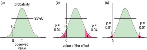
available as a docx here. IntroductionWhen researchers study a sample, they obtain an estimate of the magnitude of an effect statistic, such as a change in a mean measure of health or performance following an intervention. With the usual but crucial assumptions about representativeness of the sample, validity of the measures, and accuracy of the statistical model, a sample of sufficiently large size yields an accurate estimate of the true or population magnitude, because repeated samples would yield practically identical estimates. Sample sizes are seldom this large, so an assertion about the true magnitude of an effect should account for the fact that the sample value is only an approximate estimate of the true value. In this article I explain how to make an assertion about the true magnitude via the usual approach of the null-hypothesis significance test (NHST) and via magnitude-based inference (MBI), an approach that has been severely criticized recently (Sainani, 2018; Sainani et al., 2019; Welsh & Knight, 2015). Although the criticisms have been addressed (Hopkins, 2019a; Hopkins & Batterham, 2016; Hopkins & Batterham, 2018), it has been suggested that MBI might be more acceptable to at least some members of the statistical community, if it were presented as hypothesis tests, along with a name change to magnitude-based decisions (MBD; Hopkins, 2019a). This article is my response to that suggestion. I include an appendix with guidelines for presenting MBD as hypothesis tests in a manuscript. For the benefit of practitioners with little formal training in statistics (myself included), I have written the article with little recourse to statistical jargon. An article more suitable for an audience of statisticians has been submitted for publication by others (Aisbett et al., 2020); for the background to that article, see my posting and other postings each side of it in the datamethods forum, updated in the In-brief item on MBD in this issue. An updated version of a slideshow first presented at the German Sport University in July 2019 is also a succinct summary of this article and the In-brief item. Inferential MethodsThe null-hypothesis significance test is the traditional approach to making as assertion about the true magnitude of an effect. In NHST, the data are converted into a sampling probability distribution for the effect (or a transformation of it), representing expected variation in the effect with repeated sampling (Figure 1). This distribution is well-defined, usually a t or z. Effect values spanning the central region of the distribution represent values that are most compatible with the sample data and the model, and the interval spanning 95% of the values is known as the 95% compatibility interval (95%CI). If the 95%CI includes zero, then the data and model are compatible with a true effect of zero, so the null hypothesis H0 cannot be rejected, as shown in Figure 1a. Figure 1b shows the same data as Figure 1a, but the region of the distribution to the left of the zero and the matching area on the other tail are shaded red. The total red area defines a probability (p) value, representing evidence against the hypothesis: the smaller the p value, the better the evidence against it. With a sufficiently small p value, you reject the hypothesis. The threshold p value is called the alpha level of the test, 0.05 for a 95%CI. The p value here is 0.04 + 0.04 = 0.08, which is >0.05, so the data and model do not support rejection of H0, and the effect is declared non-significant. Not shown in Figure 1 is the limiting case, when one limit of the interval touches zero, and p = 0.05. Figure 1c shows another study of an effect where the data and model are not compatible with an effect of zero: the 95%CI does not include zero; equivalently the p value is <0.05 (0.01 + 0.01 = 0.02), so H0 is rejected, and the effect is declared significant.
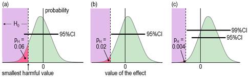
When an effect is not significant, researchers usually conclude that the true effect is trivial, insubstantial, or sometimes even zero ("there is no effect"). With small sample sizes, such a conclusion is often unjustified, which is easy to demonstrate by considering the compatibility interval: it will often be wide enough to include substantial values of the effect statistic, implying that substantial values are compatible with the data and model, so the researcher obviously cannot conclude that the effect is definitively trivial or zero. Unjustified conclusions occur also with large sample sizes: here, a significant effect is sometimes interpreted as substantial, yet the compatibility interval might include only trivial values. Dissatisfaction with misinterpretations arising from NHST has led some researchers and statisticians to focus on the compatibility interval for making an assertion about the true magnitude of an effect. Magnitude-based inference (MBI) is one such method. In MBI, the compatibility interval is interpreted as a range for the true value of the effect. A compatibility interval that includes substantial values of opposite sign is regarded as inadequate precision or unacceptable uncertainty for characterizing the true magnitude, and the effect is therefore deemed unclear. Clear effects have adequate precision, and the sampling distribution provides probabilistic estimates for reporting the true magnitude: possibly harmful, likely trivial, very likely positive, and so on. Probabilistic assertions about the true magnitude of an effect are in the domain of Bayesian statistics, so MBI is essentially, although not fully, a Bayesian method. For an analysis to be fully Bayesian, the researcher includes a prior belief in the magnitudes and uncertainties of all the parameters in the statistical model, which, together with the sample data and a sophisticated analysis, provide a posterior probability distribution and credibility interval for the true effect. However, an acceptable simplified semi-Bayesian analysis can be performed by combining the compatibility interval of an effect with a prior belief in the value of the effect statistic, itself expressed as a compatibility interval (Greenland, 2006). When a realistic weakly informative prior is combined in this manner with an effect derived from a study with a small sample size typical of those in sport and exercise research (and with any larger sample size), the resulting posterior distribution and credibility interval are practically identical to the compatibility interval and sampling distribution (Hopkins, 2019b; Mengersen et al., 2016). The probabilistic statements of MBI are therefore effectively Bayesian statements for a researcher who would prefer to impose no prior belief in the true value of an effect. Formally, MBI is reference Bayesian, with a prior that is so dispersed as to be practically uniform over the range of non-negligible likelihood, and thus only weakly informative relative to the likelihood function (S. Greenland, personal communication). When sample sizes are small, researchers should check that a realistic weakly informative prior does indeed make no practical difference to the compatibility interval, as noted in the article (Hopkins, 2019b) on Bayesian analysis with a spreadsheet. If a weakly informative prior results in noticeable "shrinkage" of either of the compatibility limits of an effect, or if the magnitude-based decision is modified by the prior, the researcher should justify such a prior and report the modified decision. Other researchers have proposed a Bayesian interpretation of the compatibility interval or the sampling distribution similar to those of MBI (Albers et al., 2018; Burton, 1994; Shakespeare et al., 2001). Some researchers interpret the compatibility interval as if it represents precision or uncertainty in the estimation of the value of an effect, but they stop short of identifying their approach as Bayesian (Cumming, 2014; Rothman, 2012). MBI differs from all these approaches by providing specific guidance on what constitutes adequate precision or acceptable uncertainty when making a decision about the magnitude of the effect. Partly for this reason, and partly because of concerns expressed about use of the word inference (Greenland, 2019), MBI is now known as a method for making magnitude-based decisions (Hopkins, 2019a). MBD nevertheless finds itself in a precarious position, pilloried by Bayesians who insist on informative priors and by frequentists who believe that science advances only in Popperian fashion by testing and rejecting hypotheses. Sander Greenland's suggestion to reframe MBD in terms of hypothesis testing was motivated by what he sees as the need for the well-defined control of error rates that underlie hypothesis testing. I have been opposed to hypothesis testing, for reasons espoused by many others, apparently as far back as Francis Bacon and Isaac Newton (e.g., Glass, 2010). My preference has been instead for estimation of the magnitude of effects and their uncertainty to make decisions about the true magnitude based on the Bayesian interpretation, but at the same time accounting for decision errors. I will now show that such decisions are equivalent to rejecting or failing to reject several hypotheses, and that the errors arising from making wrong decisions are the same as the errors with hypothesis testing. Clinical MBD and the Hypothesis of HarmIn a clinical or practical setting, it is important that the outcome of a study does not result in implementation of an intervention that on average could harm the population of interest. The hypothesis that the true effect is harmful is therefore a more relevant hypothesis to reject than the hypothesis that the true effect is zero (the standard null). Figure 2, adapted from Lakens et al. (2018), shows distributions, compatibility intervals and one-sided p values associated with the test of the hypothesis H0 that the true effect is harmful, for three different outcomes that could occur with samples. Formally, the test of the harmful hypothesis is a non-inferiority test, in which rejection of the hypothesis of inferiority (harm) implies the effect is non-inferior (e.g., Castelloe & Watts, 2015).
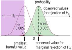
Harmful values are anything to one side of the smallest harmful value, and since this value is negative in the figure, harmful values are anything to the left of this value. Positive harmful values (e.g., a threshold blood pressure for hypertension) would fall to the right of a smallest harmful positive value. The test of the hypothesis that the effect is any harmful value belongs to the class of one-sided interval hypothesis tests. The important point about such tests is that harmful values are compatible with the sample data and model, when the compatibility interval includes harmful values, so the hypothesis of harm is rejected only when the interval does not include such values. Figure 2 shows examples of p values for the test, pH. The threshold pH value for rejecting the hypothesis is the area of the distribution on one tail to the left of the compatibility interval of a chosen level: 0.025 or 0.005 for 95% or 99% respectively. These threshold or alpha values, expressed as percents, define maximum error rates for rejecting the hypothesis of harm, when the true effect is the smallest harmful, as shown in Figure 3 for a threshold pH value of 0.005.
The error rate is set by the researcher through the choice of level of compatibility interval or threshold p value, similar to the way the error rate is set for rejecting the null hypothesis in NHST. The error rates are independent of sample size. The error for rejecting the null is Type 1, but here it is Type 2, since the hypothesis rejected is for a substantial (harmful) true effect. To avoid further confusion, I prefer to call the error a failed discovery: in making the error, the researcher fails to discover that the effect is harmful. When a compatibility interval overlaps harmful values, the true effect could be harmful, to use the Bayesian interpretation of the interval. Furthermore, the p value for the test of harm and the probability that the true effect is harmful in MBD are defined by the sampling distribution in exactly the same way. In the clinical version of MBD, a clinically relevant effect is considered for implementation only when the probability that the true effect is harmful is <0.005 (<0.5%); this requirement is therefore equivalent to rejecting the hypothesis of harm with pH<0.005 in a one-sided test. MBD is apparently still the only approach to inferences or decisions in which an hypothesis test for harm, or equivalently the probability of harm, is the primary consideration in analysis and in sample-size estimation. An important issue therefore is whether pH<0.005 represents sufficient evidence against the hypothesis of harm. To properly address this issue could involve quantitative evaluation of the perceived and monetary cost of harm, along with the cost-effectiveness of potential benefit arising from implementing the effect as a treatment in a specific setting. A threshold of 0.005 is divorced from consideration of costs and was chosen to represent most unlikely or almost certainly not harmful (Hopkins et al., 2009), which seems a realistic way to describe something expected to happen only once in more than 200 trials. For another interpretation of low probabilities, Greenland (2019) recommends converting p values to S or "surprisal" values. The S value is the number of consecutive heads in fair coin tossing that would have the same probability as the p value. The S value is given by ‑log2(p), and with pH=0.005, the value is 7.6 head tosses. Saying that the treatment is not compatible with harmful values (pH<0.005) corresponds to saying that there is more information against the hypothesis of harm than there is information against fairness in coin tossing when you get seven heads in a row (S. Greenland, personal communication). The only other researchers to devise a qualitative scale for probabilities comparable with that of MBD is the Intergovernmental Panel on Climate Change (IPCC), who deem p<0.01 (i.e., S>6.6) to be exceptionally unlikely (Mastrandrea et al., 2010). With a probability threshold for harm of half this value, MBD is one coin toss more conservative. MBD is also effectively more conservative about avoiding harm than Ken Rothman's approach to precision of estimation. In his introductory text on clinical epidemiology (Rothman, 2012), he refers to 90% confidence intervals three times more often than 95% intervals, and he does not refer to 99% intervals at all. Clinical MBD and the Hypothesis of BenefitMaking a
decision about implementation of a treatment is more than just using a
powerful test for rejecting the hypothesis of harm (and thereby ensuring a
low risk of implementing a harmful effect, to use the Bayesian
interpretation). There also needs to be consideration that the treatment
could be beneficial. Once again, a one-sided test is involved, formally a
non-superiority test, in which rejection of the hypothesis of superiority
(benefit) implies the effect is non-superior (Castelloe
& Watts, 2015). See Figure 4.
With the same
reasoning as for the hypothesis of harm, a compatibility interval that falls
short of the smallest beneficial value implies that no beneficial values are
consistent with the data and model (or in the Bayesian interpretation, the
chance that the true effect is beneficial is too low), so you would not
implement it (Figure 4a). A compatibility interval that overlaps beneficial
values allows for beneficial values to be compatible with the sample and
model (or for the possibility that the true effect is beneficial, to give the
Bayesian interpretation), so you cannot reject the hypothesis that the effect
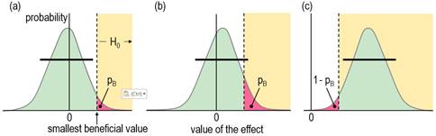
is beneficial, so it could be worth implementing (Figure 4b and 4c). Figures
4a and 4b show the p value for the test of benefit, pB.
Figure 4c shows the p value for the test of the hypothesis that the effect is
not beneficial, 1 – pB: in this example, the compatibility
interval falls entirely in the beneficial region, so the hypothesis of non-benefit is rejected. What level should the researcher choose for the compatibility interval and the associated threshold pB value in the test of the beneficial hypothesis? The level 50% was chosen via the Bayesian interpretation of a compatibility interval that just touches the beneficial region: the area of the tail overlapping into beneficial values is the probability that the true effect is beneficial, and a 50% compatibility interval has a one-sided 25% tail, which was considered a lower threshold for possibly beneficial. In other words, one should consider an effect to be possibly or potentially beneficial and implementable, provided there is a sufficiently low risk of harm. A threshold or alpha pB value of 0.25 implies an error rate of 25% for failing to discover the smallest beneficial effect (which can be shown with a figure similar to Figure 3). While this error rate may seem high, it is comparable with the 20% Type-2 error rate that underlies the calculation of sample size in conventional null-hypothesis testing. The calculation provides a sample size that would give statistical significance for 80% of studies, or a failed-discovery rate of 20%, when the true effect is the minimum clinically important difference (the smallest beneficial value). Of course, researchers are free to specify a lower threshold pB to reduce the rate of failing to discover benefit (here, failing to reject benefit), but a lower error rate comes with a cost. For example, if the threshold pB is 0.05, equivalent to one tail of a 90% compatibility interval, a tail overlapping into the beneficial region with an area of only 6% is regarded as failure to reject the beneficial hypotheses, or from the Bayesian perspective, an observed quite trivial effect with a chance of benefit of only 6% is potentially implementable. Furthermore, a trivial true effect on the margin of smallest important would have a 95% rate of failure to reject the beneficial hypothesis, a very high false-discovery or Type-1 error rate (see below), assuming harm had been rejected. There is also a problem with requiring a high chance of benefit for implementation, as shown in Figure 4c, which depicts a test resulting in rejection of the hypothesis that the effect is not beneficial. This is the approach of superiority or minimum-effects testing (MET), promoted by researchers who would prefer to reject an hypothesis of non-benefit rather than failure to reject the hypothesis of benefit (e.g., Lakens et al., 2018). If the threshold p value for this test is 0.05 (for a one-sided 90% interval), a smallest important beneficial effect would be implemented only 5% of the time (a failed-discovery or Type-2 error rate of 95%), regardless of the sample size! In an attempt to address this problem, the sample size in MET is chosen to give a low failed-discovery rate for an "expected" true effect somewhat greater than the smallest important. For example, with a p-value threshold of 0.05 for rejecting the hypothesis of non-benefit, a simple consideration of sampling distributions similar to those in Figure 3 shows that the minimum desirable sample size for MBD would give a failed-discovery rate of 50% for a true effect that is 2× the smallest important, but the rate is only 5% for a true effect that is 3× the smallest important, which is borderline small-moderate in all my magnitude scales (Hopkins, 2010). The minimum desirable sample size in MBD should therefore satisfy those who promote sample-size estimation for MET. In any case, and regardless of sample size, the hypothesis test underlying MET is automatically available in MBD, as explained below. Hypotheses for Non-Clinical MBDI have presented the clinical version of MBD above as two one-sided hypothesis tests. The tests for harm and benefit have to differ in their respective threshold p values, because it is ethically more important to avoid implementing a harmful effect than to fail to implement a beneficial effect. The non-clinical version of MBD can also be recast as one-sided tests, but now the threshold p values are the same, because rejecting the hypothesis of a substantial negative effect is just as important as rejecting the hypothesis of a substantial positive effect. A p value of 0.05, corresponding to one tail of a 90% compatibility interval, was chosen originally for its Bayesian interpretation: rejection of the hypothesis of one of the substantial magnitudes corresponds to a chance of <5% that the true effect has that substantial magnitude, which is interpreted as very unlikely. As already noted, Ken Rothman uses the 90% level for confidence intervals three times more frequently than the 95% level, so in this respect non-clinical MBD is similar to his approach. Geoff Cumming, the other researcher interpreting confidence intervals in terms of precision of estimation, uses the 95% level as a default (Cumming, 2014), so his approach is more conservative than non-clinical MBD. Combining the HypothesesAn unclear outcome in non-clinical and clinical MBD corresponds to failure to reject both hypotheses of substantiveness: the relevant compatibility intervals span both smallest important values. The Bayesian interpretation of an unclear clinical effect is that the true effect could be beneficial and harmful, while an unclear non-clinical effect could be substantially positive and negative. The interpretation of could depends on the relevant threshold p values: MBD defines could be harmful to mean pH>0.005, so the risk of harm is at least very unlikely; could be beneficial means pB>0.25, so the chance of benefit is at least possibly; could be substantial means p+>0.05 and p–>0.05, or chances of both magnitudes are at least unlikely. When the true value of an effect is substantial of a given sign, the outcome consistent with this effect is failure to reject the hypothesis of that sign and rejection of the hypothesis of opposite sign. A feature of MBD is the level of evidence it conveys for the hypothesis that could not be rejected. For example, if the hypothesis of benefit is not rejected (and harm is rejected), the effect is reported with the probabilistic terms possibly, likely, very likely or most likely preceding beneficial. Each of these Bayesian terms has an equivalent p-value threshold for testing an hypothesis that the effect is not beneficial: <0.75, <0.25, <0.05 and <0.005 respectively, and with a p value pNB = 1 – pB. The red shaded area in Figure 4c illustrates a pNB value of about 0.04, resulting in rejection of the non-beneficial hypothesis (pNB<0.05), and corresponding to very likely beneficial. This outcome is equivalent to a superiority or minimum-effects test in which the non-superiority hypothesis has been rejected at the 0.05 level. If the highest threshold for this test in MBD (pNB<0.75) seems to represent unacceptably weak evidence, keep in mind that it is equivalent to failure to reject benefit at the 0.25 threshold (pB>0.25). This weak level of evidence of benefit is captured appropriately by possibly (or, as discussed below, ambiguously). Even so, a practitioner could decide to implement a treatment with this level of evidence, given a sufficiently low risk of harm, but additional considerations are representativeness of the sample, validity of the measures, accuracy of the statistical model, cost of implementation, individual differences in the response to the treatment, and risk of side effects. For clear effects that are possibly trivial and possibly substantial (including beneficial or harmful), I suggest presenting the effect as possibly substantial, regardless of which probability is greater, although stating that the effect is also possibly trivial would emphasize the uncertainty. Effects with adequate precision that are at least likely trivial can be presented as such in tables of results, without mention of the fact that one of the substantial magnitudes is unlikely while the other is at least very unlikely. Rejection of both substantial hypotheses implies a decisively trivial effect, which occurs when the compatibility interval is contained entirely within the trivial range of values. In non-clinical MBD with a 90% interval, this scenario represents an equivalence test, with the non-equivalence hypothesis rejected at the 0.05 level. Thus MBD also includes equivalence testing. A minor point here is that a decisively trivial effect can sometimes be likely trivial; for example, a 90%CI falling entirely in the trivial region, with p– = 0.03 and p+= 0.04, implies pT = 1 – (p– + p+) = 0.93, which is likely trivial. Very likely trivial effects are, of course, always decisively trivial. In clinical MBD rejection of the beneficial hypothesis (pB<0.25) and harmful hypothesis (pH<0.005) can result in a clear effect reported as possibly trivial, which should not be regarded as decisively trivial. Sample-size EstimationA substantial rate of unclear outcomes with a small sample size is ethically problematic, since a study should be performed only if there is a publishable quantum, regardless of the true magnitude of the effect. For this reason, an interval that just fits the trivial region is the basis for minimum desirable sample-size estimation in MBD (Hopkins, 2006): a sample size any smaller produces a wider interval that could overlap both substantial regions, resulting in failure to reject both hypotheses and therefore an unclear outcome. In frequentist terms, marginal rejection of both substantial hypotheses is the basis of estimation of the minimum desirable sample size in MBD. Equally, the MBD sample size ensures a low error rate represented by deciding that a true marginally substantial effect of a given sign could be substantial of the other sign. For a marginally harmful true effect, the error rate is 0.5% for deciding that the true effect could be beneficial (failure to reject the beneficial hypothesis, with pB>0.25); for a marginally substantial negative true effect, the error rate is 5% for deciding that the true effect could be substantially positive (failure to reject the substantial positive hypothesis, with p+>0.05). Aisbett et al. (2020) have suggested sample-size estimation based on minimal-effects (superiority) testing (MET) or equivalence testing (ET). I have already shown above that the MBD sample size is consistent with that of MET for the reasonable expectation of a marginally small-moderate effect, so there is no need to replace the MBD sample size with a MET sample size. In ET, the researcher needs a sample size that will deliver a decisively trivial outcome (by rejection of the non-trivial hypothesis), if the true effect is trivial. As in MET, the researcher posits an expected value of the true effect, but now the value has to be somewhat less than the smallest important. Unfortunately, the resulting ET sample size turns out to be impractical: if the researcher posits (unrealistically) an expected true effect of exactly zero, a simple consideration of sampling distributions similar to those in Figure 3 shows that the sample size needs to be 4× that of MBD to deliver a decisively trivial outcome. A more realistic expected trivial effect midway between zero and the smallest important requires a sample size 16× that of MBD. Such large sample sizes are rarely achievable, and in any case, justification of an expected trivial true effect seems to me to be arbitrary and problematic. Showing that an effect is decisively trivial must therefore be left to a meta-analysis of many studies, and even then the effect may not be decisively trivial or substantial, if it falls close to the smallest important. I therefore see no need for a new method of sample-size estimation for MBD, but I have updated my article (Hopkins, 2020) and spreadsheet for sample-size estimation to include MET and ET. New TerminologyFor researchers who dispute or wish to avoid the Bayesian interpretation of evidence for or against magnitudes in MBD, frequentist terms have been suggested, corresponding to p-value thresholds for rejection of the one-sided hypothesis tests: most unlikely, very unlikely, unlikely, and possibly correspond to rejection of an hypothesis with p<0.005, <0.05, <0.25, and <0.75 (or failure to reject at the 0.25 level, i.e., p>0.25), which are deemed to represent strong, moderate, weak, and ambiguous rejection, respectively (Aisbett et al., 2020). The Bayesian terms describing an effect as being possibly, likely, very likely, and most likely a certain magnitude correspond to rejection of the hypothesis that the effect does not have that magnitude with p<0.75 (or failure to reject, p>0.25), <0.25, <0.05 and <0.005, which are deemed to represent ambiguous, weak, moderate and strong compatibility of the data and model with the magnitude. Greenland favors the frequentist terminology, including the use of compatibility interval rather than confidence or uncertainty interval, because "the 'compatibility' label offers no false confidence and no implication of complete uncertainty accounting" (Gelman & Greenland, 2019). Whatever the terminology, researchers should always be aware of Greenland's cautions that decisions about the magnitude of an effect are based on assumptions about the accuracy of the statistical model, validity of the measures, and the representativeness of the sample. Practitioners should also be careful not to confuse a decision about the magnitude of the mean effect of a treatment with the magnitude in individuals, who may have responses to the treatment that differ substantially from the mean. Failure to account for individual responses in the analysis of the mean effect would itself represent a violation of the assumption of accuracy of the statistical model. Use of the term unclear seems justified when neither hypothesis is rejected. Indecisive and inconclusive are also reasonable synonyms. Effects otherwise have adequate precision or acceptable uncertainty and are potentially publishable, to the extent that rejection of an hypothesis represents a quantum of Popperian evidence. However, use of the term clear to describe such effects may be responsible in part for misuse of MBI, whereby researchers omit the probabilistic term describing the magnitude and present it as if it is definitive (Lohse et al., 2020; Sainani et al., 2019). An effect that is clear and only possibly substantial is obviously not clearly substantial. Researchers must therefore be careful to distinguish between clear effects and clear magnitudes: they should refer to a clear effect as being clearly substantial or clearly trivial, when the effect is very likely or most likely substantial or trivial (moderately or strongly compatible with substantial or trivial). This use of clearly (or decisively or conclusively) for substantial magnitudes is consistent with the definition of Type-1 errors in non-clinical MBD. Type-1 Errors in MBDTo clarify the
meaning of Type-1 error, I use the term to refer to a false positive or false
discovery: the researcher makes a false discovery of a substantial
effect. In NHST a Type-1 error occurs
when a truly null effect is declared significant. Since significant is interpreted as substantial,
at least for the pre-planned sample size, the definition was broadened to
include any truly trivial effect that is declared to be substantial (Hopkins
& Batterham, 2016). This new definition allows an equitable
comparison of Type-1 rates in MBD with those in NHST. In clinical MBD,
failure to reject the hypothesis of benefit is regarded as sufficient
evidence to implement the effect. A Type-1 error therefore occurs, if the
true magnitude of the effect is trivial. With a threshold p value of 0.25,
Type-1 error rates approach 75% for trivial true effects that are just below
the smallest beneficial value, depending on sample size (Hopkins
& Batterham, 2016). For comparison, Type-1 error rates with
conventional NHST approach 80% for such marginally trivial true effects, when
sample size approaches that for 80% power and 5% significance (Hopkins
& Batterham, 2016); for greater sample sizes the error rate
exceeds 80% for conventional NHST but levels off at 50% for conservative
NHST. NHST fares better
than clinical MBD when the effect is truly null, because the NHST Type-1
error rate for such effects is fixed at 5%, whereas the rate in MBD is not
fixed and can be as high as 17%, depending on the sample size (Hopkins
& Batterham, 2016). The majority of these errors occur as
only possibly or likely beneficial, so the practitioner
opting to implement the effect should be in no doubt about the modest level
of evidence for the effect being beneficial (Hopkins
& Batterham, 2016). The Type-1 error rates are even higher in the less conservative odds-ratio version of clinical MBD, according to which an unclear effect is declared potentially implementable, if there is a sufficiently high chance of benefit compared with the risk of harm (an odds ratio of benefit to harm greater than a threshold value of 66, derived from the odds for marginally beneficial and marginally harmful). Again, the errors occur mainly as possibly or likely beneficial (Hopkins & Batterham, 2016), but the practitioner needs to take into consideration loss of control of the error in rejecting the harmful hypothesis and therefore the increased risk of implementing a harmful effect. In non-clinical MBD, a Type-1 error occurs when the true effect is trivial and the 90% compatibility interval falls entirely outside trivial values (Hopkins & Batterham, 2016): a clearly substantial effect in the new terminology. The equivalent frequentist interpretation of this disposition of the compatibility interval is rejection of the hypothesis that the effect is not substantially positive (say), with p<0.05. Rejection of this hypothesis automatically entails rejection of the hypothesis that the effect is trivial, because "not substantially positive" includes all trivial values. The Type-1 error rate in the worst case of a marginally trivial-positive true effect is at least 5%, because there is a small contribution to the error rate from compatibility intervals that fall entirely in the range of substantial negative values. Simulations with the smallest of three sample sizes (10+10) in a controlled trial showed that the error rate did not exceed 5% (Hopkins & Batterham, 2016). These simulations were performed for standardized effects using the sample SD to standardize, and the resulting compatibility intervals for deciding outcomes were based on the t distribution and therefore were only approximate. I have now repeated the simulations using the population SD to simulate a smallest important effect free of sampling error; I obtained a Type-1 error rate of 5.8% for a sample size of 10+10 (and 6.6% for a sample size of 5+5). These error rates are obviously acceptable. It is important to reiterate here that an error occurs in hypothesis testing only when an hypothesis is rejected erroneously. As already noted, in NHST a Type-1 error occurs if the true effect is zero and the null-hypothesis is rejected. Similarly, in non-clinical MBD a Type-1 error occurs if the true effect is trivial and the trivial hypothesis is rejected. Rejection of the trivial hypothesis occurs when the compatibility interval covers only substantial values, the corresponding Bayesian interpretation being that the true effect is very likely substantial. Therefore possibly substantial or likely substantial outcomes, be they publishable or unclear, represent failure to reject the trivial hypothesis and therefore do not incur a Type-1 error, a crucial point that the detractors of MBI have not acknowledged (Sainani, 2018, 2019; Sainani et al., 2019; Welsh & Knight, 2015). Janet Aisbett (personal communication) suggested that "an error of sorts also occurs when you fail to reject a hypothesis that you should have." In other words, the outcome with a truly substantial effect should be rejection of the non-substantial hypothesis, and if you fail to reject that hypothesis, you have made an error. A similar error occurs with failure to reject the non-trivial hypothesis, when the true effect is trivial. Janet's suggestion is just another way of justifying sample size with MET or ET, which I have already dealt with. It is also important to emphasize that there is no
substantial upward publication bias, if the criterion for publication of
effects with MBI is rejection of at least one hypothesis, even with quite
small sample sizes (Hopkins & Batterham, 2016). It follows that MBD offers
researchers the opportunity to publish their small-scale studies without
compromising the literature. MBD actually benefits
the literature, because several small-scale studies add up to a large study
in a meta-analysis. These assertions do not amount to an endorsement of such
studies; researchers should obviously aim for sample sizes that will avoid
unclear outcomes. Lower P-value Thresholds?The non-clinical p-value threshold of 0.05 for testing the hypothesis of a true substantial effect seems to be an appropriate threshold for very unlikely, when considered as one event in 20 trials. In terms of S values, 0.05 seems less conservative, because it represents only a little more than four heads in a row when tossing a coin. Would a lower p value threshold and consequent lower error rates for non-clinical effects be more appropriate? One of the advantages of retaining 0.05 is that the resulting estimates of sample size for non-clinical effects are practically the same as for clinical effects (Hopkins, 2006). If this threshold were revised downward, non-clinical sample size would be greater, which seems unreasonable, so the probability thresholds in clinical MBD would also need revising downwards. For example, if all the p-value thresholds were halved, their S values would move up by one coin toss. For non-clinical MBI very unlikely (0.05 or 5%) would become 0.025 or 2.5% (S = 5.3). For clinical MBI most unlikely (0.005 or 0.5%) would become 0.0025 or 0.25%, and possibly (0.25 or 25%) would become 0.125 or 12.5% (S = 8.6 and 3.0). Sample size for clinical and non-clinical MBD would still be practically the same, but they would rise from the existing approximately one-third to about one-half those of NHST for 5% significance and 80% power. A lower p-value threshold for non-clinical effects would reduce the Type-1 error rates for such effects, but a lower pB would increase the Type-1 rates for deciding that trivial true effects could be beneficial. Lower p values require bigger effects for a given sample size, so there could be a risk of substantial bias for publishable effects with lower threshold p values, when the sample size is small. Unclear effects would also be more common and therefore less publishable with some of the unavoidably small sample sizes in sport and exercise science. On balance, I recommend keeping the existing probability thresholds. A Practical Application of MBDA colleague who is skeptical about claims of performance enhancement with the substances banned by the International Olympic Committee recently asked me to evaluate an article reporting the results of a placebo-controlled trial of the effects of injections of recombinant human erythropoietin (rHuEPO) on performance of cyclists (Heuberger et al., 2017). The authors concluded that "although rHuEPO treatment improved a laboratory test of maximal exercise, the more clinically relevant submaximal exercise test performance and road race performance were not affected." The net effect of rHuEPO on mean power in the submaximal test (a 45-min trial) was presented as 5.9 W (95%CI -0.9 to 12.7 W, p=0·086), so their conclusion about performance in this test was based presumably on what appeared to be a negligible increase in mean power and, of course, statistical non-significance, along with the claim that their study was "adequately powered". Effects on endurance performance are best expressed in percent units, and for elite cyclists the smallest important change in mean power in time-trial races (defined as winning an extra medal in every 10 races on average) is 1.0% (Malcata & Hopkins, 2014). I calculated the net effect on power in the submaximal time trial as 1.1%. When I inserted these values into the frequentist and Bayesian versions of the spreadsheet for converting a p value to MBD (Hopkins, 2007), the 90%CI was 0.1 to 2.1%, and the non-clinical decision was a small, possibly (or ambiguously) positive effect (p+ = 0.54, p– = 0.001). The effect was also potentially implementable (possible benefit with really low risk of harm), but a clinical decision would be relevant only for someone considering implementation for an advantage in competitions, which is not an issue here. The road-race performance was measured only once for each cyclist, after the period of administration of rHuEPO. The authors presented the difference in the mean race time of the two groups in percent units, but without time in a pre-intervention race for comparison, the uncertainty accommodates huge negative and positive effects (0.3%, 95%CI ‑8.3 to 9.6%). The conclusion that the submaximal test and road race performance were not affected by injections of rHuEPO is obviously not tenable. The researchers assumed that non-significance implies no real effect, which is a reasonable assumption with the right sample size. Unfortunately their approach to estimating sample size left the study underpowered for the submaximal test (as shown by non-significance for an observed substantial effect) and grossly underpowered for road race performance (as shown by huge compatibility limits). Use of MBD leads to a realistic conclusion about the uncertainty in the magnitude of the effects. ConclusionIf researchers heed the recent call to retire statistical significance (Amrhein et al., 2019), they will need some other hypothesis-based inferential method to make decisions about effects, especially in clinical or practical settings. I have shown that the reference-Bayesian probability thresholds in the magnitude-based decision method are p-value thresholds for rejecting hypotheses about substantial magnitudes, which are assuredly more relevant to real-world outcomes than the null hypothesis. Researchers can therefore make magnitude-based decisions about effects in samples, confident that the decisions have a sound frequentist theoretical basis and acceptable error rates. I recommend continued use of the probabilistic terms possibly, likely, and so on to describe magnitudes of clear, decisive or conclusive effects (those with acceptable uncertainty), since these terms can be justified with either reference-Bayesian analyses or hypothesis tests, and they convey uncertainty in an accessible manner. The terms clearly, decisively or conclusively should be reserved for magnitudes that are very likely or most likely trivial or substantial: those with moderate or strong compatibility with the magnitude. Acknowledgements: I thank Janet Aisbett for
important corrections and suggestions for inclusion of additional material.
Alan Batterham and Daniel Lakens helped me understand one-sided interval
hypothesis tests. ReferencesAisbett J, Lakens D, Sainani KL. (2020). Magnitude based
inference in relation to one-sided hypotheses testing procedures. SportRxiv, https://osf.io/preprints/sportrxiv/pn9s3/. Amrhein V, Greenland S,
McShane B. (2019). Retire statistical significance. Nature 567, 305-307. Castelloe J, Watts D.
(2015). Equivalence and noninferiority testing using sas/stat® software.
Paper SAS1911-2015, 1-23 (https://support.sas.com/resources/papers/proceedings15/SAS1911-2015.pdf). Cumming G. (2014). The new
statistics: why and how. Psychological Science 25, 7-29. Hopkins WG. (2006).
Estimating sample size for magnitude-based inferences. Sportscience 10,
63-70. Hopkins WG. (2018). Design
and analysis for studies of individual responses. Sportscience 22, 39-51. Hopkins WG. (2019a). Magnitude-based
decisions. Sportscience 23, i-iii. Hopkins WG. (2020).
Sample-size estimation for various inferential methods. Sportscience 24,
17-27. Lohse K, Sainani K, Taylor
JA, Butson ML, Knight E, Vickers A. (2020). Systematic review of the use of “Magnitude-Based
Inference” in sports science and medicine. SportRxiv, https://osf.io/preprints/sportrxiv/wugcr/. Mastrandrea MD, Field CB,
Stocker TF, Edenhofer O, Ebi KL, Frame DJ, Held H, Kriegler E, Mach KJ, et
al. (2010). Guidance note for lead authors of the IPCC fifth assessment
report on consistent treatment of uncertainties. Intergovernmental Panel on
Climate Change (IPCC), https://pure.mpg.de/rest/items/item_2147184/component/file_2147185/content. Rothman KJ. (2012).
Epidemiology: an Introduction (2nd ed.). New York: OUP. Sainani KL. (2019).
Response. Medicine and Science in Sports and Exercise 51, 600. Appendix: Reporting MBD in JournalsIn the section of a manuscript dealing with statistical analysis, there should first be a description of the model or models providing the effect statistics. This description should include characterization of the dependent variable, any transformation that was used for the analysis, and the predictors in the model. For mixed models, the random effects and their structure should be described. There should be some attention to the issue of uniformity of effects and errors in the model. If a published spreadsheet was used for the analysis, cite the most recent article accompanying the spreadsheet. Following the description of the statistical model, there is a section on the MBD method that will depend on whether the journal requires hypothesis testing or accepts instead, or as well, a Bayesian analysis. Journals should be more willing to accept the original Bayesian version of MBD, now that it is clear that MBD is isomorphic with an acceptable frequentist version. Suggested texts for this section are provided below, preceded by advice on presentation of results of MBD analyses. A final paragraph on statistical analysis can deal with evaluation of observed magnitudes. Suggested text for this paragraph, which is the same for both kinds of journal, is also provided below. Journals
requiring hypothesis testing The editor should be satisfied if the p value for the usual null-hypothesis test is replaced by the p values for the one-sided tests of substantial magnitudes. Report the p values to three decimal places if ≥0.995 (e.g., 0.997), to two decimal places if ≥0.10 (e.g., 0.63), and with one significant digit if <0.10 (e.g., 0.003). Do not report the p values as inequalities. For clinical effects, the p values for the hypotheses of
harm and benefit could be presented as pH and pB.
The p values for non-clinical effects that have negative and positive
smallest important values could be p– and p+, whereas p↓
and p↑ could be used for factor effects derived via log
transformation. These p values should be accompanied by the observed effect,
the compatibility interval or limits (preferably 90%), and a qualitative
description of the observed magnitude (small, moderate, etc.). Inclusion of
the term unclear is appropriate
when both hypotheses are not rejected. The term clear can be used to describe effects when at least one
hypothesis has been rejected. Clear
or clearly can also be used to
describe the magnitude of a clear
effect (substantial or trivial), provided the p value for that magnitude is
>0.95; for example, "there was a moderate clear reduction in risk of
injury (hazard ratio 0.63, 90%CI 0.46 to 0.86, pH=0.002, pB=0.97)."
The pB of 0.97 in this example has a
frequentist interpretation of moderately
compatible with benefit,
which could be included for editors who require strictly frequentist
reporting; the Bayesian interpretation of very
likely beneficial could be included or replace pB
for editors who are comfortable with non-informative or weakly informative
priors. If you or the editor want an informative prior, the probabilities of
the true magnitudes will differ from the p values. In tables, show a column
headed by pH/pT/pB (or p–/pT/p+,
or p↓/pT/p↑), with values such as
0.03/0.05/0.92. To save numeric clutter in a table and highlight evidence for
magnitudes, clear effects (those with acceptable uncertainty) can be
indicated by using the asterisk and superscript 0 system described below for
Bayesian reporting, with the Bayesian terms replaced by the frequentist
compatibility terms. Decode the asterisks and superscripts in the table's
footnote. Methods section for a strictly frequentist journal. Uncertainty in the estimates of effects is presented as 90% compatibility intervals [or limits]. Decisions about magnitudes accounting for the uncertainty were based on hypothesis tests for substantial and trivial effects (reference: this article and/or Aisbett et al., 2020). For clinically or practically relevant effects (which could result in implementation of a treatment), hypotheses of harm and benefit were rejected if the respective p values (pH and pB) were less than 0.005 and 0.25 (strong and weak rejection, respectively). For all other effects, hypotheses of substantial decrease and increase were rejected if their respective p values (p– and p+, or for factor effects, p↓ and p↑) were less than 0.05 (moderate rejection). If only one hypothesis was rejected, the effect is described as being ambiguously, weakly, moderately or strongly compatible with the other magnitude when the p value for the test of that magnitude was >0.25, >0.75, >0.95 and >0.995, respectively. The p values for the above tests were areas of the sampling distribution of the effect statistic to the left or right of the smallest important value (the trivial-small threshold) [and were provided by the Sportscience spreadsheet in percent units as chances of benefit and harm, or substantially positive and negative]. Effects with at least one substantial hypothesis rejected and at least weakly compatible evidence with trivial magnitudes (pT >0.75) are presented as such, where pT is the p value for the test of the trivial hypothesis (the area of the sampling distribution covering trivial values). When the p value for the test of a substantial or trivial magnitude was >0.95, the magnitude is described as clear. The sampling distribution was assumed to be a t distribution for effects derived from a continuous dependent variable, or a z distribution for effects derived from counts or events [modify this sentence for your study]. Where the model providing the effects involved a log or other transformation, the smallest important value was also transformed for evaluation of the p values. P-value thresholds for rejecting the main pre-planned hypothesis in this study [describe it] were not adjusted for the inflation of error that occurs with multiple inferences. For the remaining tests, thresholds were divided by n [state it; a default for study with many effects could be 10], to give a Bonferroni-type correction equivalent to n independent tests. Effects with hypotheses thus rejected are highlighted in bold in tables and figures; to reduce inflation of error, interpretation of outcomes is focused on these effects. Minimum desirable sample size was estimated for Type-2 (failed-discovery) error rates set by the p-value thresholds (0.5% and 25% for smallest important harmful and beneficial clinical effects respectively; 5% for substantial negative and positive non-clinical effects) using a spreadsheet (Hopkins, 2006). [Use smaller error rates where relevant for multiple inferences.] Error of measurement [for sample-size estimation of controlled trials and crossovers] was estimated from previously published similar studies [state references for the studies] using the panel of cells for that purpose in the spreadsheet. Methods section incorporating hypothesis tests and Bayesian analysis. Uncertainty in the estimates of effects is presented as 90% compatibility intervals [or limits]. Decisions about magnitudes accounting for the uncertainty were based on hypothesis tests for substantial and trivial effects (reference: this article and/or Aisbett et al., 2020). For clinically or practically relevant effects (which could result in implementation of a treatment), hypotheses of harm and benefit were rejected if the respective p values (pH and pB) were less than 0.005 and 0.25 (strong and weak rejection, respectively). For all other effects, hypotheses of substantial decrease and increase were rejected if their respective p values (p– and p+, or for factor effects, p↓ and p↑) were less than 0.05 (moderate rejection). If only one hypothesis was rejected, the p value for the other hypothesis corresponds to the posterior probability of the magnitude of the true (large-sample) effect in a reference-Bayesian analysis with a minimally or weakly informative prior (Hopkins, 2019b), so it was interpreted with the following scale: >0.25, possibly; >0.75, likely; >0.95, very likely; >0.995, most likely (Hopkins et al., 2009). [Provide additional text here if an informative prior was used, or if the sample size was so small that a weakly informative prior modified the magnitude-based decision; state that the modified decision is presented (Hopkins, 2019b).] If neither hypothesis was rejected, the effect is described as unclear, with the exception of effects with an odds ratio of benefit to harm >66, which were considered clear and potentially implementable. The p values for the above tests were areas of the sampling distribution of the effect statistic to the left or right of the smallest important value (the trivial-small threshold) [and were provided by the Sportscience spreadsheet in percent units as chances of benefit and harm, or substantially positive and negative]. Effects with at least one substantial hypothesis rejected and at least likely trivial magnitudes (pT >0.75) were presented as such, where pT was the p value for the test of the trivial hypothesis (the area of the sampling distribution covering trivial values). When the p value for the test of a substantial or trivial magnitude was >0.95, the magnitude is described as clear. The sampling distribution was assumed to be a t distribution for effects derived from a continuous dependent variable, or a z distribution for effects derived from counts or events [modify this sentence for your study]. Where the model providing the effects involved a log or other transformation, the smallest important value was also transformed for evaluation of the p values. Include here the two paragraphs on adjustment for multiple inferences and sample-size estimation described above for a strictly frequentist journal. Journals
accepting Bayesian analysis If you opt for informative priors, be sure to justify them and to show the point estimate, compatibility interval and MBD before and after application of the prior for the most important effects. Unclear effects should be presented without a probabilistic term, but otherwise show possibly, likely, and so on, usually after the observed magnitude. Examples: small unclear harmful; moderate likely beneficial; large very likely substantial increase; possibly trivial-small positive (if trivial and substantial positive are both possible). Clear or decisive can be used to describe such effects, but refer to clearly substantial or clearly trivial only for very likely or most likely substantial or trivial. Examples: clearly trivial; a large clear increase. To save space in a table, substantial effects can be indicated with ↓ or ↑, and the probabilistic terms for substantial effects can be replaced (with an appropriate explanatory footnote) by *, **, ***, and **** for possibly, likely, very likely, and most likely substantial; for trivial effects, use 0, 00, 000, and 0000. Examples: large↓****; small↑**; trivial00; small↑ (for an observed small but unclear increase). A possibly trivial possibly substantial effect can be indicated accordingly, to emphasize the uncertainty. Examples: trivial0↓* (if the observed effect was trivial, possibly trivial and possibly negative); small↓*,0 (if the observed effect was small, possibly negative and possibly trivial). Methods section. Uncertainty in the estimates of effects is presented as 90% compatibility intervals [or limits]. Decisions about magnitudes accounting for the uncertainty were based on a reference-Bayesian analysis with a minimally informative prior (Hopkins, 2019a; Hopkins & Batterham, 2016; Hopkins & Batterham, 2018), which provided estimates of chances that the true magnitude was harmful, trivial and beneficial (for clinically or practically relevant effects, which could result in implementation of a treatment), or chances that the true magnitude was a substantial decrease or negative value, a trivial value, and a substantial increase or positive value (for all other effects). [Provide additional text here if an informative prior was used, or if the sample size was so small that a weakly informative prior modified the magnitude-based decision; state that the modified decision is presented, with the chances from the posterior distribution (Hopkins, 2019b).] Clinically relevant effects were deemed clear (had adequate precision) if the risk of harm was <0.5%, or the chances of benefit were <25%, or the odds ratio of benefit to harm was >66; non-clinical effects had adequate precision if the chances of one or other substantial true value were <5% (the 90% compatibility interval did not include substantial positive and negative values). Clear effects are reported with a qualitative descriptor for the magnitudes with chances that are >25% using the following scale: >0.25, possibly; >0.75, likely; >0.95, very likely; >0.995, most likely (Hopkins et al., 2009). When the chances of a substantial or trivial magnitude were >95%, the magnitude itself is described as clear. Effects with inadequate precision are described as unclear. [If you make ~10 or more decisions about magnitudes, and you do not opt for the exact Bonferroni correction for inflation of error described below, make the following statement here.] Effects with adequate precision defined by 99% compatibility intervals are highlighted in bold in tables and figures; the overall error rate for coverage of 10 independent true values with such intervals is that of a single effect with a 90%CI (10%), and interpretation of outcomes is focused on these effects. The chances of substantial and trivial magnitudes of the true effect were the percent areas of the sampling distribution of the effect statistic to the left or right of the smallest important value (the trivial-small threshold). The sampling distribution was assumed to be a t distribution for effects derived from a continuous dependent variable, or a z distribution for effects derived from counts or events [modify this sentence for your study]. Where the model providing the effects involved a log or other transformation, the smallest important value was also transformed for evaluation of the chances of magnitudes. The threshold chances of substantial magnitudes for deciding adequate precision of the magnitude of the main pre-planned effect in this study [describe it] were not adjusted for inflation of error that occurs with multiple decisions. For all other decisions, threshold chances were divided by n [state it], to give a Bonferroni correction equivalent to n independent decisions. Effects with adequate precision following correction are highlighted in bold in tables and figures; to reduce inflation of error, interpretation of outcomes is focused on these effects. Minimum desirable sample size was estimated for adequate precision in the limiting cases of maximum acceptable risk of harm for minimum acceptable chance of benefit (0.5% and 25% for smallest important harmful and beneficial clinical effects respectively) and maximum acceptable chance of substantial negative and positive non-clinical effects (5% for smallest important negative and positive) using a spreadsheet (Hopkins, 2006). [Use smaller values where relevant for multiple inferences.] Error of measurement [for sample-size estimation of controlled trials and cross-overs] was estimated from previously published similar studies [state references for the studies] using the panel of cells for that purpose in the spreadsheet. Magnitude scales
for all journals Here is suggested text for a paragraph on scales for assessing magnitudes. Delete the information about scales that are not in your study… All effects are presented with the qualitative magnitude of their observed (sample) value, evaluated with the following scales for trivial, small, moderate, large, very large and extremely large respectively (Hopkins et al., 2009): for effects with no known relationship to performance, wealth or health, standardized thresholds given by <0.2, ≥0.2, ≥0.6, ≥1.2, ≥2.0, and ≥4.0 times the appropriate between-subject standard deviation [which you will have to describe in the section devoted to the modeling]; Pearson correlation coefficients of <0.1, ≥0.1, ≥0.3, ≥0.5, ≥0.7, and ≥0.9, corresponding to these standardized thresholds; for effects on or directly related to competitive performance times or distances, an increase or decrease of <0.3, ≥0.3, ≥0.9, ≥1.6, ≥2.5, and ≥4.0 times the within-athlete variability of performance between major competitions (analyzed as percent effects via log transformation) [you will have to state this value and cite a publication for it]; for individual or team match performance, <1, ≥1, ≥3, ≥5, ≥7, and ≥9 extra wins or losses in every 10 matches with an otherwise evenly matched opponent (analyzed via logistic models); for effects on injury or other morbidity or mortality prevalence or incidence, on counts, or on wealth, factor decreases of >0.9, ≤0.9, ≤0.7, ≤0.5, ≤0.3, and ≤0.1, and factor increases represented by their reciprocals, <1.11, ≥1.11, ≥1.43, ≥2.0, ≥3.3, and ≥10. To evaluate magnitudes of standard deviations representing variability in an effect (individual differences or responses), the square of the standard deviation was assumed to be normally distributed (Hopkins, 2018), and the magnitude thresholds are one-half of those in the above scales, equivalent to evaluating two standard deviations with the above thresholds (Smith & Hopkins, 2011). Effects of between- or within-subject linear numeric predictors were evaluated for two between- or within-subject standard deviations of the predictor, representing typically high minus typically low predicted effects (Hopkins et al., 2009). First published 8 June 2020. |